PROM-trends plot function

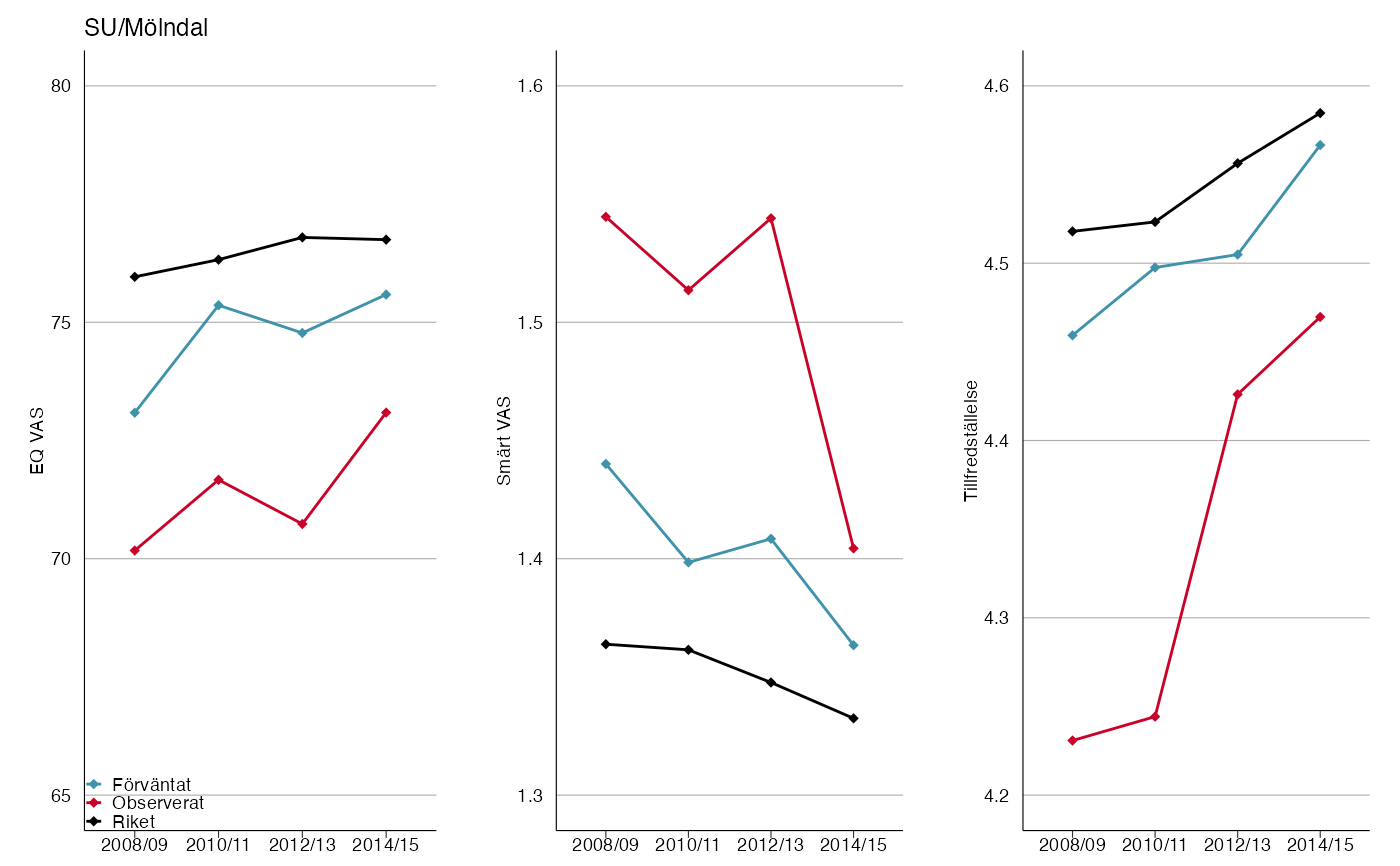
Visualizing PROM-trends for each clinic using ggplot2.

prom_trends(
  eq_vas_exp,
  eq_vas_obs,
  eq_vas_riket,
  pain_exp,
  pain_obs,
  pain_riket,
  satis_exp,
  satis_obs,
  satis_riket,
  riket_name = "Riket",
  y_labs = c("EQ VAS", "Smärt VAS", "Tillfredställelse"),
  y_breaks = c(5, 5, 5),
  year = c("2008/09", "2010/11", "2012/13", "2014/15"),
  subset = 1,
  legend_labels = c("Förväntat", "Observerat", "Riket"),
  line_colors = c("#3E92AA", "#C90327", "black"),
  line_size = 0.5,
  point_size = 1.5,
  legend.position = c(0, 0),
  n_row = 1,
  n_col = 3,
  ...
)

Arguments

eq_vas_exp

Data frame with expected EQ VAS data.

eq_vas_obs

Data frame with observed EQ VAS data.

eq_vas_riket

Data frame with Swedish average EQ VAS data.

pain_exp

Data frame with expected pain VAS data.

pain_obs

Data frame with observed pain VAS data.

pain_riket

Data frame with Swedish average pain VAS data.

satis_exp

Data frame with expected satisfaction VAS data.

satis_obs

Data frame with observed satisfaction VAS data.

satis_riket

Data frame with Swedish average satisfaction VAS data.

riket_name

Character to find what row is Swedish average, usually named "Riket".

y_labs

Labels for y-axis

y_breaks

Y breaks in the three plots.

year

X-axis years, character vector works. The year variables will be renamed as they appear in the data set.

subset

Which plots should be generated, subset = 1 corresponds to the first plot in alphabetical order.

legend_labels

Labels for the legends in the plot.

line_colors

Colors of the lines.

line_size

Line thickness of the lines in plot.

point_size

Point sizes in plot.

legend.position

Position of the legend in plot, matrix where each row corresponds to a legend position is recommended, if length(subset) > 1.

n_row, n_col

Number of rows/columns for the three plots.

...

arguments passed to theme_slr()

Value

List of several gtable objects where each gtable object is one clinic

Examples

# Create trend plot for SU/Mölndal
# Look at 9 data sets to see the required structure.
p <-
  prom_trends(
  shprplotfun::eq_vas_exp,
  shprplotfun::eq_vas_obs,
  shprplotfun::eq_vas_riket,
  shprplotfun::pain_exp,
  shprplotfun::pain_obs,
  shprplotfun::pain_riket,
  shprplotfun::satis_exp,
  shprplotfun::satis_obs,
  shprplotfun::satis_riket,
  y_breaks = c(5, 0.1, 0.1),
  subset = 49
)
#> Warning: Package 'extrafont' not installed!
#>             This might cause problems with fonts if you export figures to PNG!

plot(p)