Sweden map data set with county included, compressed version

Sweden map data set with county included, compressed version

swe_landsting

Format

A data frame with 7,791 rows and 19 variables. This is a filtered version of swe_landsting_allpoints where all points with piece equal to "3" or larger are removed (small details) and only every thirtieth point being used (see examples). Also some example variables are included for example purposes, calculated for 2016 annual report.

NAME_1

name of county, character

id

id of county, character

long

longitude, numeric

lat

latitude, numeric

order

specifies the order for each point, integer

piece

"1" for the most essential, "2" and more for detailed points (Öland, Orust, and Tjörn included in "2"), factor

group

Each region or island in the map is a polygon where each level in this variable is a polygon, factor

VARNAME_1

alternative name of county, character

cat_eq5d

Preoperative EQ5D*

cat_eqvas

Preoperative EQ VAS*

cat_pain

Preoperative Pain VAS*

cat_eq5d_post

Postoperative EQ5D*

cat_eqvas_post

Postoperative EQ VAS*

cat_pain_post

Postoperative Pain VAS*

cat_sati_post

Postoperative Satisfaction VAS*

cat_eq5d_dev

Postoperative adjusted EQ5D*

cat_eqvas_dev

Postoperative adjusted EQ VAS*

cat_pain_dev

Postoperative adjusted Pain VAS*

cat_sati_dev

Postoperative adjusted Satisfaction VAS*

* Factor variable with 3 levels for counties compared to the interval \((\mu - \sigma, \mu + \sigma\) where \(\mu\) and \(\sigma\) are the mean and standard deviation for whole Sweden: bad (below the interval), average (within) and good (above).

Examples

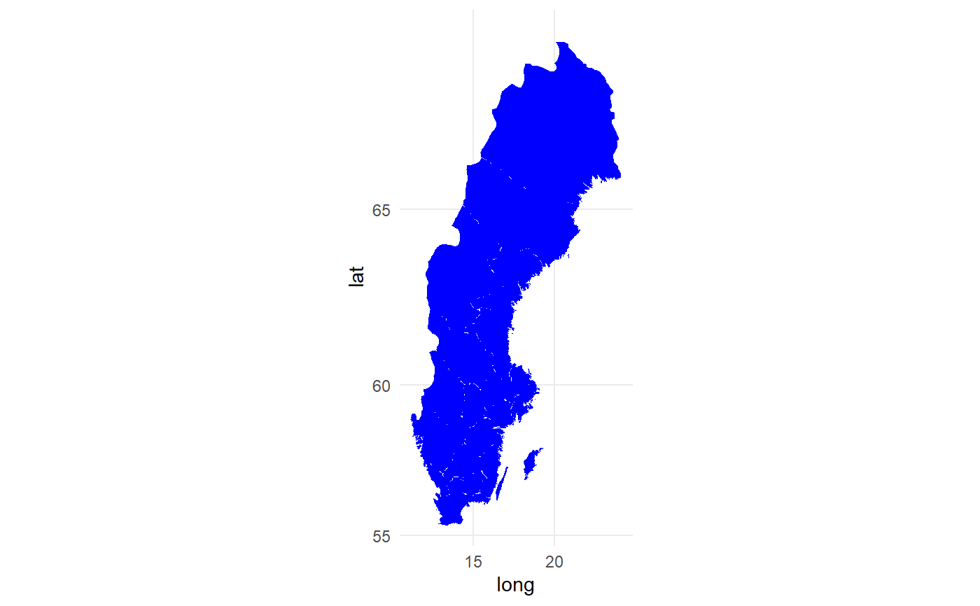
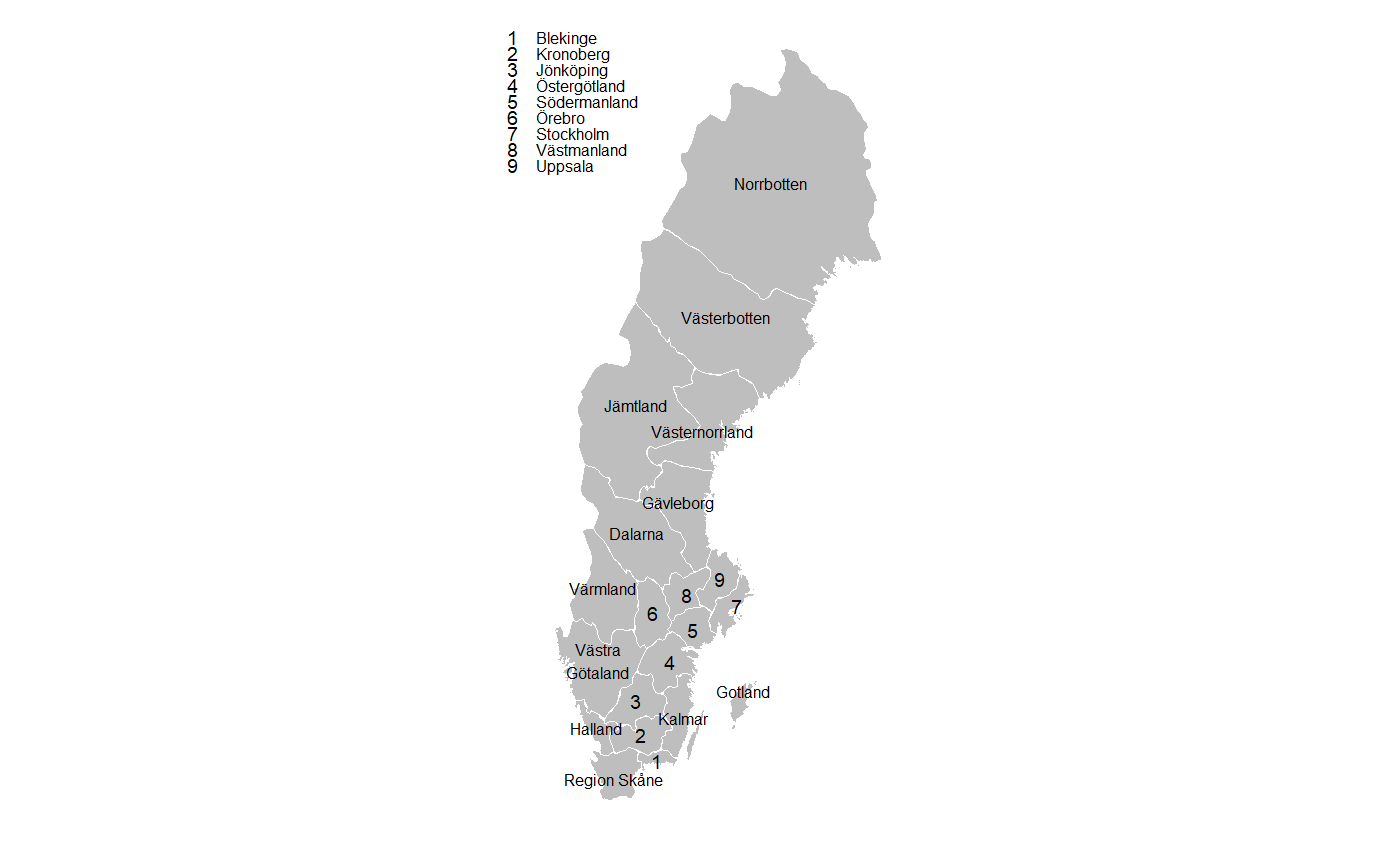
# How swe_landsting_allpoints was filtered

swe_example <-
  dplyr::filter(swe_landsting_allpoints,
  piece %in% c("1", "2")) %>%
  dplyr::filter(order %% 30 == 1) %>%
  droplevels()

# Example on how to make map of Sweden using ggplot2.
# Note that coord_map() is essential for the map to be in actual scale.

ggplot2::ggplot(
  data = swe_landsting,
  ggplot2::aes(x=long, y=lat, group = group)
) +
ggplot2::geom_polygon(color = "transparent", fill = "blue") +
ggplot2::coord_map() +
ggplot2::theme_minimal()

# Example on how to make a nice Sweden map with text guides.

ggplot2::ggplot(
  data = swe_landsting,
  ggplot2::aes(x=long, y=lat, group = group)
) +
ggplot2::geom_polygon(color = "white", size = 0, fill = "grey")  +
ggplot2::geom_point(
  data = cnames1,
  ggplot2::aes(x = long, y = lat, group = NAME_1, shape = NAME_1),
  size = 6 * 0.352777778,
  color = "black"
) +
ggplot2::scale_shape_manual(
  values = as.character(1:9),
  guide = ggplot2::guide_legend(ncol = 1)
) +
ggplot2::geom_text(
  data = cnames2,
  ggplot2::aes(x = long, y = lat, group = NAME_1, label = as.character(NAME_1)),
  size = 6 * 0.352777778,
  color = "black",
  hjust = 0.5
) +
ggplot2::coord_map() +
ggplot2::theme_minimal() +
ggplot2::xlab("") +
ggplot2::ylab("") +
ggplot2::theme(
  plot.title           = ggplot2::element_blank(),
  axis.text            = ggplot2::element_blank(),
  axis.title.x         = ggplot2::element_text(size = 8, color = "black"),
  axis.title.y         = ggplot2::element_text(size = 8, color = "black"),
  panel.grid           = ggplot2::element_blank(),
  panel.background     = ggplot2::element_blank(),
  axis.ticks           = ggplot2::element_blank(),
  legend.text          = ggplot2::element_text(size = 6),
  legend.title         = ggplot2::element_blank(),
  legend.key.height    = ggplot2::unit(6, "pt"),
  legend.key.width     = ggplot2::unit(6, "pt"),
  legend.position      = c(-0.13,1),
  legend.justification = c(0,1),
  plot.margin          = ggplot2::margin(0,0,0,0, unit = "cm")
)