PROM-trends plot function

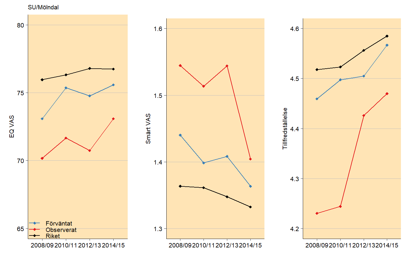
Visualizing PROM-trends for each clinic using ggplot2.

prom_trends(
  eq_vas_exp,
  eq_vas_obs,
  eq_vas_riket,
  pain_exp,
  pain_obs,
  pain_riket,
  satis_exp,
  satis_obs,
  satis_riket,
  riket_name = "Riket",
  y_labs = c("EQ VAS", "Smärt VAS", "Tillfredställelse"),
  y_breaks = c(5, 5, 5),
  year = c("2008/09", "2010/11", "2012/13", "2014/15"),
  subset = 1,
  text_size = 8,
  legend_labels = c("Förväntat", "Observerat", "Riket"),
  line_colors = c("#377EB8", "#E41A1C", "black"),
  background_color = "moccasin",
  panel_grid_color = "grey",
  panel_grid_size = 0.3,
  axis_size = 0.3,
  line_size = 0.5,
  point_size = 1.5,
  legend_pos = c(0, 0),
  n_row = 1,
  n_col = 3
)

Arguments

eq_vas_exp	Data frame with expected EQ VAS data.
eq_vas_obs	Data frame with observed EQ VAS data.
eq_vas_riket	Data frame with Swedish average EQ VAS data.
pain_exp	Data frame with expected pain VAS data.
pain_obs	Data frame with observed pain VAS data.
pain_riket	Data frame with Swedish average pain VAS data.
satis_exp	Data frame with expected satisfaction VAS data.
satis_obs	Data frame with observed satisfaction VAS data.
satis_riket	Data frame with Swedish average satisfaction VAS data.
riket_name	Character to find what row is Swedish average, usually named "Riket".
y_labs	Labels for y-axis
y_breaks	Y breaks in the three plots.
year	X-axis years, character vector works. The year variables will be renamed as they appear in the data set.
subset	Which plots should be generated, subset = 1 corresponds to the first plot in alphabetical order.
text_size	Text size in pt.
legend_labels	Labels for the legends in the plot.
line_colors	Colors of the lines.
background_color	Color of the panel background.
panel_grid_color	Color of the panel grid lines.
panel_grid_size	Size of the panel grid lines in plot, useful to change if large dpi!
axis_size	Size of the axis lines, useful to change if large dpi
line_size	Line thickness of the lines in plot.
point_size	Point sizes in plot.
legend_pos	Position of the legend in plot, matrix where each row corresponds to a legend position is recommended, if length(subset) > 1.
n_row, n_col	Number of rows/columns for the three plots.

Value

List of several gtable objects where each gtable object is one clinic

Examples

# Create trend plot for SU/Mölndal
# Look at the 9 data sets to see the required structure.
# Data sets are included in the package.

example_plot <- prom_trends(
  eq_vas_exp, eq_vas_obs, eq_vas_riket, pain_exp,
  pain_obs, pain_riket, satis_exp, satis_obs, satis_riket,
  y_breaks = c(5, 0.1, 0.1), subset = 49)

plot(example_plot)